SPoRT Embarks on a Project to Produce Stream Height Forecasts using Machine Learning

The use of various soil moisture parameters from the SPoRT-LIS for monitoring drought conditions and assessing flood risk has been ongoing for years, and has been demonstrated for efficacy at other collaborative offices.  The use of soil moisture output for drought analysis is relatively straight-forward.  However, the use of the data for assessing flood risk has always been a bit more complicated and has involved the development of significant thresholds of rainfall and soil moisture that lead to flooding based on forecaster experience.  This method lends itself to some degree of subjectivity and has always been less quantitatively robust than preferred.  Nevertheless, the SPoRT-LIS data have provided valuable information regarding the state of soil moisture and the potential for flooding in near real-time.  There are older posts on the blog that describe the application of the data for flood risk assessment.

Now, the SPoRT group is embarking on a new project, employing a machine learning technique to provide a more quantitative measure of the relationship between soil moisture values, rainfall and stream height.  This new methodology involves the use of a Long Short-Term Memory (LSTM) Network.  The LSTM model for a particular drainage basin can be trained using a history of SPoRT-LIS soil moisture values, gauge height observations, and precipitation from the Multi-Radar Multi-Sensor Quantitative Precipitation Estimation data set.  Using this training data set, the forecast model for each basin is then run in real-time using the most recent gauge height observations, SPoRT-LIS soil moisture at various depths, and quantitative precipitation forecasts (QPF).  For this initial version of the gauge height forecasts, we’re using QPF values from the GFS model and the WPC.  One of the advantages of this type of modeling is that the great majority of computational power is on the front-end to train the model, while running the model in real-time is computationally much less expensive than running a hydrologic model.  Thus, we can run multiple precipitation scenarios for any basin quickly in real time.  For example, for the 40+ basins in our initial evaluation, the amount of processing time needed to run each basin at 6-hourly time steps out to 5 days with two different precipitation schemes takes just about 5 minutes!

The SPoRT group is working with some of our collaborative NWS offices (Huntsville, Nashville, Morristown, Sterling) and the Lower Mississippi and Mid-Atlantic River Forecast Centers (LMRFC and MARFC, respectively) for this initial test and evaluation of the stream height forecasts.  Although SPoRT has produced models for several thousand basins in the Southeast CONUS domain, this initial evaluation will involve a sub-set of streams, shown in the image below.

Image 1.  Gauge locations (black dots) for the initial evaluation of real-time gauge height forecasts from NASA SPoRT.

So, one might be asking…why is SPoRT engaged with stream height forecasting?  It’s important to remember that the SPoRT paradigm involves working closely with collaborative partners and assessing forecaster needs.  One of those needs involves having a better sense of flood risk at mid to long timescales during the 7-day forecast period.  Let us explain.  Operational gauge height forecasts from the RFC may not incorporate precipitation into the hydrologic models beyond one or two days due to operational and model limitations and constraints.  However, this can be problematic if an area is expecting heavy rainfall in the period beyond a day or two.  Take for example the current flooding event occurring across parts of the Tennessee Valley.  Operational gauge height forecasts for the Flint River (at Brownsboro, AL) from the afternoon of February 3rd indicated no rise forecast for the river (Image 2).  This is because the hydrologic models were not incorporating precipitation into the models as it was before the 48 hour cutoff.

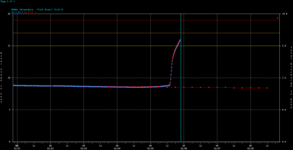
Image 2.  Graph of gauge height observations (dotted blue line) and forecasts (dotted red line) for the Flint River at Brownsboro.  The forecast was valid approximately 1440 UTC 3 Feb 2020.  Observations are current through about 22 UTC 5 Feb 2020.  Horizontal bars at the top of the image indicate flooding thresholds (yellow=Action Stage, orange=Minor Flood, red=Moderate Flood)

However, heavy rain was expected in the region, which would certainly lead to some river rises.  The question is…how much?  Our old rules of thumb would have suggested flooding likely, based on soil moisture values and expected rainfall.  But again, the old rules didn’t indicate the time frame for flooding or the degree of flooding…it was generally just a qualitative “likely” or “not likely”.  So, to help alleviate this gap in knowledge, the new methodology provides objective, deterministic forecasts of stream or gauge height.  The image below shows the gauge height forecasts from the SPoRT LSTM models valid at about the same time.  Notice that the forecasts based on both GFS and WPC QPF scenarios indicated flooding was likely, while the higher precipitation from the GFS suggested flooding would reach Moderate Stage.  So, it’s easy to see here one of the advantages this type of modeling can have for overall hydrologic forecasting and situational awareness for the threat of flooding.

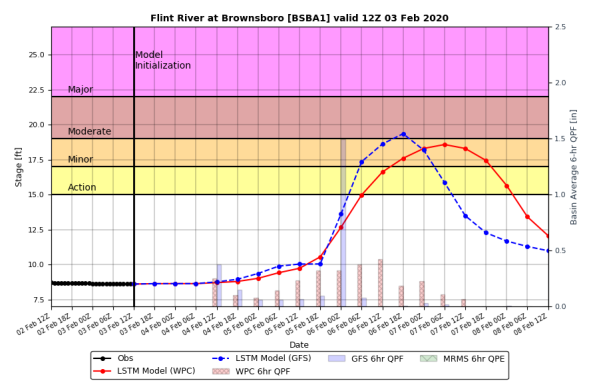
Figure 3.  SPoRT LSTM gauge height forecasts for the Brownsboro River at Brownsboro.  The black line shows observations, up to analysis time at 12Z 3 Feb 2020.  The blue dashed line contains gauge height forecasts based on GFS QPF, while the red line contains forecasts based on WPC QPF.  The blue vertical bars indicate 6-hourly GFS QPF, while the red bars indicate 6-hourly WPC QPF.

This post has become rather long.  So, we’re going to leave it here for now.  We’ll be providing more information about this project and discussing other advantages and limitations of our stream height forecasts in some upcoming posts as we continue this evaluation over the next couple of months.

– Kris and Andrew

Wide disparity in soil wetness this summer across Alabama and the Southeastern U.S.

The pattern of soil moisture across the state of Alabama and more broadly the Southeastern United States has evolved into one of marked disparity over relatively short distances (see Fig. 1d) and time frames. The SPoRT Center manages its own instance of the NASA Land Information System (i.e., “SPoRT-LIS”), which produces real-time soil moisture estimates in an observations-driven modeling framework.  Hourly and daily output fields are available on the SPoRT Center web page, and 3-hourly and daily data are delivered to select NOAA/NWS weather forecast offices for enhanced decision support in areas such as drought and hydrologic applications.

In general, 2019 has been quite a wet year across large portions of the U.S., with parts of Alabama being no exception (especially northwestern Alabama).  Beginning in May, a rapid deterioration in soil wetness occurred across many parts of the Southeast due to unusually hot and dry conditions during the last half of May through early June.  However, the latter part of June into July featured well above-average rainfall in some areas that reversed the rapid drying trends, especially over far northwestern Alabama, Mississippi, and western Tennessee.  The variations in SPoRT-LIS total-column soil moisture percentiles over the past 4 months are given in Fig. 1, illustrating the regional spatiotemporal trends described above from April through July.

Fig 1. Monthly-evolving, total-column SPoRT-LIS soil moisture percentiles (relative to a 1981-2013 climatology) over the Southeastern U.S., valid (a) 30 Apr, (b) 31 May, (c) 30 Jun, and (d) 31 Jul 2019. [Click on image for full resolution]

Interestingly, the soil moisture percentiles across far northern Alabama diminish quite substantially from west to east by the end of July (Fig. 1d), approaching the 98^th percentile in western Lauderdale county (NW Alabama) to less than the 10^th percentile across Jackson county (NE Alabama; counties of northern Alabama shown in Fig. 2).  The current conditions on 31 July 2019 relative to the 31 July historical soil moisture distributions from a 1981-2013 SPoRT-LIS daily climatology further illustrate this sharp zonal contrast in soil wetness anomalies within the county-based histograms of Fig. 3. The county-mean 0-2 meter relative soil moisture on 31 July 2019 in Lauderdale county is at the 87^th percentile compared to the 33-year historical distribution of 31 July values (Fig. 3a).  Meanwhile, Limestone county to its east has a mean soil moisture at the 61^st percentile (Fig. 3b), followed by the 51^st percentile in Madison county (Fig. 3c) and only the 24^th percentile in Jackson County, AL.  These results serve to illustrate the highly variable nature of rainfall and resulting soil wetness and agricultural impacts that can occur across the Southeastern U.S. during the summer months.

Fig 2. Counties of northern Alabama. The far northern counties of Lauderdale, Limestone, Madison, and Jackson are highlighted within the discussion text and in Figure 3.

Fig. 3.  Historical distributions of 0-2 meter relative soil moisture on 31 July and present-day county means on 31 July 2019 for all SPoRT-LIS grid points within a specific county, valid for far northern Alabama counties ranging west to east from (a) Lauderdale, (b) Limestone, (c) Madison, and (d) Jackson.  Gray bars represent the frequency distributions of 1981-2013 soil moisture values, vertical colored lines are reference percentiles, and the black dashed lines are present-day, county-averaged soil moisture value, with values tabulated in the upper-right of each panel. [Click on image for full resolution]

Finally, despite the month-to-month swings in soil moisture anomalies across much of the Southeast in recent months, one corridor that has persistently experienced abnormally dry conditions extends from southeastern Alabama into southern and central Georgia and western South Carolina. In fact, since 31 May (Figs. 1b-d), southeastern Alabama has seen soil moisture percentiles less than 20%, analogous to moderate to severe (or worse) proxy drought categories based on community-accepted conventions of percentile anomalies.  These dry regional pockets in the SPoRT-LIS analysis strongly correspond to the most recent U.S. Drought Monitor weekly product, issued on 30 July (Fig. 4).

Fig 4.  U.S. Drought Monitor weekly product valid for the week of 30 July 2019.

 

SPoRT LIS Shows Dry Soils During High Plains Blowing Dust Event…

Yesterday while working on some Dust RGB related training materials, I was looking at the RGB in AWIPS and noticed a dust event unfolding in real-time in the central High Plains.  The loop below shows Dust RGB imagery, generated by GOES-East, yesterday, 28 Jan 2019 during the late morning and early afternoon hours.  The loop is centered over NE Colorado and SW Nebraska where you’ll see the blowing dust develop and spread southeastward.  In case you’re not too familiar with this type of imagery, the dust is represented by the magenta colors.  It’s also possible to observe some of the individual dust streaks or plumes within the larger blowing dust event, which help to show their locations of origin.  (By the way, sorry about the loss of image fidelity when saving from AWIPS to an animated GIF).

Image 1.  GOES-East Dust RGB imagery, approx. 1737-2002 UTC, 28 Jan 2019. The blowing dust is defined by the magenta colors, near the center of the imagery.

Research has shown that it takes the right combination of factors to loft dust particles sufficiently to generate these larger scale blowing dust events, partly based on soil moisture and winds.  The SPoRT LIS 0-10 cm volumetric soil moisture (VSM) analysis at 18 UTC indicated very low values in the blowing dust source region, with VSM percentages generally around 12-16% (Image 2).  The METAR observations also indicate sustained winds were 35-40 knots with stronger gusts over 40 knots at one locations in the area.

Image 2. SPoRT LIS volumetric soil moisture (background colors) overlaid with surface METAR plots (yellow figures), valid at 18 UTC, 28 Jan 2019.

This last image is a snapshot of the Dust RGB taken at 1902 UTC, overlaid with surface visibility and ceiling observations.  Notice that at station KHEQ in far northeastern Colorado, a ceiling of 100 ft and visibility of 7 SM was reported, which was likely due to the blowing dust.

Image 3. GOES-East Dust RGB and ceiling and visibility observations from ground observation stations at approximately 19 UTC, 28 Jan 2019.

Some SPoRT collaborative NWS offices in the West CONUS have utilized LIS VSM values to locate areas where the probability of blowing dust events is heightened under the proper conditions.  However, SPoRT is looking into opportunities to better predict where these events will occur.

SPoRT LIS Shows Low Soil Moisture Conditions Near Large N. Cal Fire…

Just making a quick post here as I noticed there were relatively dry soil moisture conditions at the site of a rather large fire that developed quickly in Butte County, CA today.  The first image is the Fire Temperature RGB from the GOES-16 satellite (mesoscale domain sector 1) at 2018 UTC, today, 8 Nov 2018.  In this RGB, the fire can be observed by  colors ranging from near red to near white, just east of Chico, CA.  Notice there are a few white pixels, indicating relatively high emissions from shorter wavelengths (1.61 µm), and thus, relatively hot fire temperatures.

Meanwhile, soil moisture data from SPoRT’s Land Information System show low soil moisture percentiles (from the 33-year climatology, next image below) at the fire’s location east of Chico.  In fact, these values are  below the 2nd percentile at the fire’s location.

Lastly, the one year change in deep layer soil moisture values (0-200 cm) also show significant decreases in soil moisture centered at the fire’s location and especially just east over the last year.

SPoRT is conducting research and working closely with members of the wildfire community in the western U.S. to transfer these and other data sets for operational decision-makers.

-Kris W.

Dramatic Soil Moisture Transformation over North Carolina Associated with Flooding Rainfall from Hurricane Florence

As anticipated, Hurricane Florence resulting in monumental rainfall totals, particularly across southern and eastern North Carolina.  This past week’s rainfall totals are depicted in Figure 1, derived from the NOAA/National Weather Service Advanced Hydrologic Prediction Service (AHPS).  Widespread totals exceeded 10” across most of southern/eastern North Carolina and far eastern South Carolina, with maximum rainfall of more than 20” along and within a few counties of the Atlantic Coast.

Figure 1.  Weekly total rainfall (inches), valid 11-18 September 2018, from the National Weather Service Advanced Hydrologic Prediction Service (AHPS) product.  Four counties are denoted, for which soil moisture histogram animations are shown later in this article.

The extreme rainfall dramatically impacted the soil moisture, which underwent a substantial transformation from very dry to near-saturation across south-eastern North Carolina.  Figure 2 shows soil moisture retrievals before and after Hurricane Florence from NASA’s Soil Moisture Active Passive (SMAP) mission, which estimates near-surface soil moisture (~top 5 cm) in near-real-time derived from passive microwave satellite observations.  A 6-day animation of hourly SPoRT-LIS simulated 0-100 cm relative soil moisture images overlaid with Multi-Radar Multi-Sensor rainfall contours (Fig. 3) nicely shows how the predominantly very dry soils across North and South Carolina prior to Florence were quickly moistened to near saturation over just a few days.  [Ongoing research at SPoRT seeks to further improve the experimental soil moisture estimates by assimilating SMAP retrievals into the SPoRT-LIS framework.]

Figure 2.  NASA Soil Moisture Active Passive (SMAP) Level 2 soil moisture retrievals from before (top panel; valid 11 September) and after Hurricane Florence (bottom panel; valid 16 September).

Figure 3.  Animation of hourly SPoRT-LIS 0-100 cm relative soil moisture images overlaid with MRMS precipitation contours, valid for the period 0000 UTC 12 Sep to 2300 UTC 17 Sep 2018. [Click on image for full resolution]

Similar to that shown in a companion blog article, Figure 4 shows the evolution of shallow (0-10 cm) to total column/deep (0-200 cm) soil moisture percentiles relative to the SPoRT-LIS 1981-2013 climatological database.  Anomalously dry soil moisture is depicted by orange/red colors, while anomalously wet soil moisture is given by green/blue colors.  Prior to Hurricane Florence, much of South Carolina and southern parts of North Carolina were experiencing unusually dry soil moisture for this time of year.  Despite the capacity for the soils to receive moisture, the historic rainfall was enough to overcome soil moisture deficits, quickly leading to near-saturated soil conditions in all model depths, and ultimately substantial flooding.  An interesting feature to note after the storm impact is the very high soil moisture percentiles greater than 98^th percentile across South Carolina in the shallow layers.  Meanwhile, the deeper soils experienced excessive soil moisture percentiles above the 98^th percentile predominantly over North Carolina where the heaviest rainfall occurred and where the pre-storm dry anomalies were not as large as in South Carolina.

Figure 4.  Daily animations of SPoRT-LIS soil moisture percentiles relative to 1981-2013 climatology, valid from 10 to 17 September over model depths at (top image) 0-10 cm, (2nd image) 0-40 cm, (3rd image) 0-100 cm, and (bottom image) total model column 0-200 cm.  [Click on each individual image for full resolution]

 

Finally, the dramatic transformation in soil moisture is nicely highlighted by examining the present-day, county-averaged values relative to the 1981-2013 climatological distributions, as shown in Figure 5 at four select counties in North Carolina.  Robeson and Cumberland counties (first and third images in Figure 5) experienced the driest soils prior to Hurricane Florence (westernmost counties in Fig. 1), whereas New Hanover and Craven counties (second and fourth images in Figure 5) were more moist prior to Florence’s rainfall.  Each of the four sampled counties ultimately experienced record daily soil moisture values by 17 September (99.9^th percentiles).  However, the moist antecedent soils in Craven county led to record soil moisture values by 15 September, whereas the other counties that began with drier soils achieved record values by 16 or 17 September.  In summary, despite predominantly dry soils prior to Hurricane Florence across much of the Carolinas, the tremendous 10-30”+ rainfall totals led to a quick saturation of the soils and massive, widespread flooding.

Figure 5. Daily animations of SPoRT-LIS total column, county-averaged soil moisture histograms, valid from 10-17 September 2018 for (top image) Robeson county, NC [city of Lumberton], (2nd image) New Hanover county, NC [city of Wilmington], (3rd image) Cumberland county, NC [city of Fayetteville], and (bottom image) Craven county, NC [city of New Bern].  Gray bars represent frequency distribution of 1981-2013 climatological 0-200 cm relative soil moisture values, vertical colored lines are reference percentiles, and black dashed line is present-day, county-averaged soil moisture value. [Click on each image for full resolution]

 

Hurricane Florence to Impact the Carolinas with Massive Rainfall

All eyes are on North and South Carolina as Major Hurricane Florence approaches the region over the next two days.  One important component to the official forecast is for the storm to slow down as it approaches the coast, due to the collapse of major atmospheric steering currents.  As a result, the NCEP Weather Prediction Center is predicting extreme rainfall amounts, especially for southeastern coastal North Carolina where 15-20”+ of rainfall is anticipated over the next 7 days (Fig. 1).

Figure 1.  NCEP Weather Prediction Center 7-day rainfall forecast, valid for the period 1200 UTC 12 September through 1200 UTC 19 September 2018. [Click image for full view]

An examination of the antecedent soil moisture is helpful to qualitatively assess the ability of the ground to absorb some of the moisture from the incoming rainfall.  Figure 2 shows a collage of shallow to deep soil moisture percentiles from 12 September within the four layers of the Noah land surface model, as being run in real time within NASA SPoRT’s configuration of the Land Information System (i.e., “SPoRT-LIS”).  The percentiles are derived from a 1981-2013 database of SPoRT-LIS daily soil moisture values in order to compare the present-day soil moisture to historical values on any given day of the year.  In Fig. 2, we see that recent soil moisture values are historically quite dry over central/northern South Carolina and into far southern North Carolina, with values under the 10^th percentile (and even 2^nd percentile, yellow/red shades) in some areas.  Meanwhile, as one traverses inland and northward, the soils steadily moisten to anomalously wet conditions (green/blue shades), especially over interior North/South Carolina to the Appalachian Mountains.

Figure 2.  SPoRT-LIS soil moisture percentiles on 12 September 2018, relative to 1981-2013 daily climatological values for the following layers: (a) 0-10 cm (top model layer), (b) 0-40 cm (top two model layers), (c) 0-100 cm (top three model layers), and (d) 0-200 cm (all four model layers). [Click image for full view]

The dry soil moisture anomalies near the coast suggest that the soils will initially be able to absorb incoming rainfall fairly effectively.  However, as prolonged heavy rainfall continues with the expected slow movement of Hurricane Florence, the soils should quickly become saturated, thereby leading to enhanced runoff and flooding potential over time.  So while having dry soils will be of some help early in the event, a prolonged exceptional rainfall up to 20”+ will lead to substantial flooding regardless of the initial soil moisture distribution.

The blog author documented a similar scenario (also over South Carolina), where substantial moisture from Hurricane Joaquin in Autumn 2015 led to 20”+ rainfall totals, largely occurring over dry soils in an area of moderate to severe drought, thereby completely eliminating the drought classification in South Carolina and producing substantial flooding.  A similar scenario was also seen associated with Hurricane Harvey in southeastern Texas last year, where very dry soils were prevalent prior to Harvey’s landfall north and west of Houston Metro.  However, given the very prolonged exceptional rainfall event, incredible soil moistening and flooding occurred anyway in much of southeastern Texas.

 

Wet streaks in soil moisture observed in west Texas…

This morning I observed some rather odd looking streaks in the 10.3 µm imagery in western portions of Texas.  Sampling the 10.3 µm data revealed alternating areas of relative warm/cool skin surface temperatures in the cloud free conditions in the area on the upstream side of departing deep convection.  The temperature difference in the skin temperatures were around 5 C at this time.  The 10.3 µm image below was taken from appox. 1357 UTC this morning (3 May 2018).

Image 1.  10.3 um imagery from GOES-16, 1357 UTC 3 May 2018

Arguably, the streaks of lower temperature values showed up better in the 3.9 µm imagery.  Notice the streaks or alternating bands of yellow/orange colors in portions of west Texas.

Image 2.  3.9 um imagery from GOES-16, 1357 UTC 3 May 2018

Realizing these temperature differences were likely due to the recent convective rainfall, I looked up the SPoRT LIS 0-10 cm volumetric soil moisture data, which corresponded nearly perfectly with the streaks of relative lower temperature values (Image 3).  So indeed, this was due to the recent heavy, convective rainfall across the area.

Image 3.  SPoRT LIS 0-10 cm Volumetric Soil Moisture, 15 UTC 3 May 2018

 

Extreme Wildfire Setup over Southern High Plains for 17 April

The fire weather outlook for today (17 April 2018) looks very dire over the Southern High Plains of western Texas, New Mexico, and portions of western Oklahoma, southwestern Kansas, and southeastern Colorado. The combination of very little precipitation in recent months along with expected strong winds and extremely low relative humidities will set the stage for potentially dangerous wildfires over this region. The NCEP Storm Prediction Center has the highest threat category in today’s fire weather outlook across the region, with a large swath of extremely critical fire weather conditions expected (Fig. 1).

The persistent lack of precipitation over the Southern High Plains and Desert Southwest regions and its impact on deep-layer soil moisture is captured by the SPoRT-LIS 6-month change in total column relative soil moisture, as posted on the SPoRT-LIS graphics web page (Fig. 2; https://weather.msfc.nasa.gov/sport/case_studies/lis_CONUS.html).  A sharp transition lies across Kansas, Oklahoma and Texas, where a strong drying signal is seen across western portions of these states into New Mexico, Arizona, and Mexico, whereas dramatic moistening is prevalent in the last 6 months over the Mississippi, Ohio, and Tennessee River Valleys.  Substantial drying is also noted over the southern Florida Peninsula, with wetting seen over the West Coast and Pacific Northwest (Fig. 2).

Since the unusual and persistent dry pattern over the Southern Plains and Desert Southwest has occurred during the winter months when vegetation is typically dormant (which taps into the deeper soil moisture layers), the anomalously dry conditions are best captured by soil moisture percentiles in the near-surface layer of the SPoRT-LIS.  The total column SPoRT-LIS soil moisture percentiles does not depict an overly dramatic anomaly over the Desert Southwest (Fig. 3; unusual dryness is most prevalent in the deep layers from Oklahoma/Kansas up to Wisconsin/Illinois); however, the shallow soil moisture percentiles capture the anomalous drying over these regions near the surface, as seen in the animation of daily 0-10 cm percentiles for April  in Fig. 4, especially over West Texas, New Mexico and Arizona.  Medium-range forecasts suggest there could be precipitation over the Southern High Plains this weekend, but numerous wetting events will be needed to relieve the ongoing drought conditions.

Figure 1. NCEP Storm Prediction Center’s Day-1 fire weather outlook map for 17 April 2018.

Figure 2. Six-month change in SPoRT-LIS total column relative soil moisture for the period ending 16 April 2018.

Figure 3. SPoRT-LIS total column relative soil moisture percentiles, valid for 16 April 2018.

Figure 4. Daily animation of top-layer (0-10 cm) SPoRT-LIS soil moisture percentiles for the period 1 April to 16 April 2018.

Assimilation of NASA Soil Moisture Active Passive (SMAP) Retrievals to Improve Modeled Soil Moisture Estimates and Short-term Forecasts

For several years, SPoRT has been running a real-time simulation of the NASA Land Information System (hereafter, “SPoRT-LIS“), over a Continental U.S. domain at a ~3-km spatial resolution.  The SPoRT-LIS product is a Noah land surface model climatological and real-time simulation over 4 model soil layers (0-10, 10-40, 40-100, and 100-200 cm). For real-time output, the Noah simulation is updated four times per day as an extension of the long-term climatology simulation.  It ingests NOAA/NESDIS daily global VIIRS Green Vegetation Fraction data, and the real-time SPoRT-LIS component also incorporates quantitative precipitation estimates (QPE) from the Multi-Radar Multi-Sensor (MRMS) gauge-corrected radar product.  The long-term, climatological SPoRT-LIS is based exclusively on atmospheric analysis input from the NOAA/NASA North American Land Data Assimilation System – version 2.

Over the last 1-2 years, SPoRT has been conducting applied research to improve its SPoRT-LIS analyses by assimilating Level 2, enhanced-resolution soil moisture retrievals from the NASA Soil Moisture Active Passive (SMAP) mission.  Comparisons between the “SMAP-LIS” (assimilating the SMAP soil moisture retrievals) and the current SPoRT-LIS (without data assimilation) are available in a near real-time research page.  Data assimilation experiments are being conducted over both Continental U.S. and East Africa domains, and the utility of SMAP data assimilation over Alaska during the warm season is being explored as well.  Besides producing more accurate soil moisture estimates, the project also seeks to improve short-term numerical weather prediction (NWP) models by comparing model runs initialized with SPoRT-LIS enhanced with SMAP data assimilation against model runs initialized with the current SPoRT-LIS soil moisture fields.  This blog post provides a status of this ongoing research, highlighting recently-published work and preliminary NWP model results.

Improvements to Modeled Soil Moisture Estimates

[The data assimilation discussion below represents an excerpt from Blankenship et al. 2018]

To reduce model forecast error in a land surface or atmospheric model, it is essential to periodically update model states with independent observations (Fig. 1).  Data assimilation methods are used to combine an existing model state (background) with a set of observations in order to produce a new model analysis.  The SMAP-LIS uses an Ensemble Kalman Filter to combine SMAP observations with the modeling capabilities of the previous SPoRT-LIS, with the goal of improving states of soil moisture , soil temperature, and fluxes of moisture and energy at the land surface.

Figure 1.  Conceptual diagram of data assimilation (DA).  The black curve represents the true state of some model variable over time at a single point.  The red curve represents a forecast unconstrained by observations and whose error grows with time.  With data assimilation, the observations (blue diamonds) are used to adjust the model value at each assimilation cycle (gray arrows), producing a new forecast (purple curve) that is closer to reality.

An important step in data assimilation is to perform a bias correction to adjust the observations to match a known model distribution.  This is desirable because the solution for the new model analysis makes the assumption that the model and observation are unbiased relative to each other.  The choice of the temporal and spatial scales for this correction are somewhat subjective.  If the initial model climatology has biases built in, e.g., a systematic wet bias or a regionally-varying bias, a strict correction to the model climatology will maintain the model’s previous bias.  Since we seek to take advantage of the global consistency of SMAP observations, we have implemented a non-local bias correction by aggregating points to generate a location-independent correction curve for each soil type (since many modeling errors are related to soil type).  Figure 2 shows the resulting correction curves for 8 broad soil-type categories.

An advantage of applying the weaker non-local constraint when performing the bias correction is that it allows SMAP to influence the climatology of the soil moisture.  We have identified some geographic model biases in our existing SPoRT LIS run, forced by NLDAS-2 analyses.  One example involves the blending of disparate US and Canadian precipitation observations in the Great Lakes region.  This blending produced a persistent dry anomaly in the southern Ontario region (between Lakes Superior, Erie, and Ontario) in the SPoRT-LIS.  This is seen in Fig. 3a, which shows the monthly average 0-100 cm soil moisture for June 2016.  The SMAP retrievals (A single overpass is shown in Fig. 3c.), while relatively dry in this region, are more consistent with nearby areas in Michigan and the northern parts of Indiana and Ohio.  (Note that the color scale is different since this figure represents the top 5 cm only.)  As the result of repeated data assimilation, the SMAP-LIS soil moistures (Fig. 3b) in Southern Ontario over the 0-100 cm layer are more consistent with those in neighboring regions to the south and west.  This example illustrates how the non-local bias correction can help correct spatially varying errors in the model soil moisture.

A quantitative validation (Table 1) was performed against a soil moisture gauge at Elora, Ontario (depicted by the star in Fig. 3c) for two summers.  Results show that the SMAP-LIS soil moistures were more accurate in terms of bias and RMSE for 2015 and 2016.  Results for unbiased RMSE, correlations, and anomaly correlations were mixed from year to year but all three metrics performed better in the second year of the experiment.

Figure 2. Bias correction curves for 8 soil type groupings used to convert SMAP retrievals to model-equivalent values.

Figure 3. Long-term impact of SMAP data assimilation on root zone soil moisture. (a) Average of 1200 UTC 0-100 cm relative soil moisture (%) for June 2016 from SPoRT-LIS (no data assimilation), (b) Same quantity but for SMAP-LIS, (c) SMAP retrieved soil moisture on 4 June 2016. (m³ m^-3 x100).  The star shows the location of a soil moisture gauge used for validation. (Click on image for full size view)

TABLE 1. Validation statistics (bias, RMSE, unbiased RMSE, correlation, anomaly correlation) from Elora, Ontario, Canada soil moisture gauge for summer 2015 (30 May-4 Sep) and summer 2016 (2 May-31 Aug).  For each pair of measurements, the better value is in bold type.

	2015		2016
Metric	SPoRT-LIS	SMAP DA	SPoRT-LIS	SMAP DA
Bias	-0.096	-0.077	-0.083	-0.043
RMSE	0.102	0.088	0.115	0.086
ubRMSE	0.036	0.042	0.079	0.075
RCORR	0.76	0.69	0.38	0.48
ACORR	0.77	0.67	0.55	0.57

Impacts on Short-term NWP Model Forecasts

The second component of this research involves compared NWP model simulations initialized with SPoRT-LIS and SMAP-Enhanced DA fields, using the NASA Unified-Weather Research and Forecasting (NU-WRF) modeling framework for the experiments.  NU-WRF simulations are currently focused on the CONUS during the warm season (May to August) to document impacts of SMAP data assimilation on short-term regional NWP.  A case study of improved timing of a mesoscale convective system (MCS) is highlighted here.  Ongoing work involves examining other high-impact convective cases during the 2015 and 2016 warm seasons, and conducting comprehensive model verification statistics.

The case highlighted here is from a severe MCS over the Midwest from 13-14 July 2016.  The NCEP/Storm Prediction Center reports from this day are available at http://www.spc.noaa.gov/climo/reports/160713_rpts.html. An MCS developed over Missouri and Illinois during the afternoon of 13 July, and quickly moved eastward into Indiana, Michigan, and Ohio and southern Ontario province into the evening.  The initial surface soil moisture differences between the SMAP-LIS and SPoRT-LIS (Fig. 4) show that a distinct drying occurred in the data assimilation output over the Midwest, compared to the SPoRT-LIS output.  Meanwhile, a moistening occurred from SMAP DA over portions of Southern Ontario, as illustrated above.  (Note that the moist “stripe” surrounding the Great Lakes is consistent with the appearance of a moist bias near coastlines found within the SMAP Enhanced Resolution Level 2 product).  A similar signal is seen in the deeper soil layers as well.

Figure 4.  Difference in initial 0-10 cm volumetric soil moisture between SMAP-LIS and SPoRT-LIS for the model runs initialized at 0000 UTC 13 July 2016.

The soil drying signal over the Midwest led to a corresponding increase in 2-m temperatures, decrease in 2-m dew points, and overall decrease in surface convective available potential energy (CAPE), as seen in the NU-WRF 18-h forecast (Fig. 5).  Meanwhile, over southern Ontario, the more moist soils in the SMAP-LIS initialized run led to an opposite response.  These changes to the simulated boundary layer environment led to an overall faster propagation of the MCS across Illinois and Indiana in the SMAP-LIS initialized NU-WRF runs, as highlighted in Fig. 6.  This faster solution was in better agreement with the observed radar reflectivity at 0000 UTC 14 July, as the NU-WRF run initialized with SPoRT-LIS data had too slow of a solution at this time.  While the two solutions converged to a slow-biased placement and timing after dark, secondary development over Southern Ontario was more aggressive in the SMAP-LIS initialized run, again in better agreement with reality (Fig. 7).  More comprehensive analysis and model verification will help us better understand the cause and effect relationship between the soil moisture initialization and the resulting NU-WRF simulation differences for this case, as well as composite results during the 2015 and 2016 warm seasons.

Figure 5.  Differences in NU-WRF simulated 2-m temperature (left panel; SMAP-Enhanced minus SPoRT-LIS), surface CAPE (middle), and 2-m dew point (right) for the 18-h forecast valid 1800 UTC 13 July 2016.  (Click on image for full size view)

Figure 6.  Comparison of NU-WRF simulated composite radar reflectivity for the (a) SPoRT-LIS initialized run, (c) SMAP-LIS initialized run, and (b) validating radar reflectivity observation, for the 24-h forecast valid 0000 UTC 14 July 2016. (click on image for full size view)

Figure 7.  Same as in Fig. 6, except for the 28-h forecast valid 0400 UTC 14 July 2016. (click on image for full size view)

Comparison of Soil Moisture Response in Hurricanes Harvey and Irma

After a record [nearly] 12 years between landfalling major hurricanes [cat 3 or higher], the United States has now experienced two major hurricanes making landfall less than three weeks apart from one another.  Hurricane Harvey brought exceptional record rainfall to southeastern Texas and southwestern Louisiana because it stalled shortly after landfall due to a lack of atmospheric steering currents.  Less than 3 weeks later, Major Hurricane Irma made landfall twice in Florida: once in the Lower Keys and again near Marco Island on the southwestern coast.  A long-lived cat 5 hurricane prior to landfall, Irma had a very large wind field which resulted in far-reaching impacts along the Florida East Coast, up to Charleston, SC, and inland to Atlanta, GA, with millions of households and businesses without electricity and/or water.

Here at the NASA SPoRT Center, we have been closely monitoring these two hurricanes through numerous social media and blog posts of unique satellite products and through SPoRT’s real-time instance of the NASA Land Information System (“SPoRT-LIS”).  This blog post serves to compare the soil moisture responses to hurricanes Irma and Harvey rainfall, as depicted by the real-time SPoRT-LIS output.  The Relative Soil Moisture (RSM) variable is shown throughout this article, since it takes into account the variations in soil composition by scaling the moisture availability between the wilting point (plants cannot uptake moisture) and saturation point (soil cannot hold any more water).  The SPoRT-LIS runs the Noah land surface model, which estimates soil moisture through 4 layers: 0-10, 10-40, 40-100, and 100-200 cm depth.  We first examine the response during Irma in the top 0-10 cm layer, followed by 0-100 cm layer for both storms, and then compare the total column (0-200 cm) values relative to historical values from a climatological database spanning 1981-2013 (33 years).

Figure 1 compares the weekly rainfall accumulation primarily from Hurricane Irma over the Southeastern U.S. to the August monthly rainfall total over Texas/Louisiana, primarily contributed from Hurricane Harvey during the final week of August. Rainfall from Irma was quite substantial in the Florida peninsula up to coastal South Carolina, where numerous locations measured over 10″ of rain in less than 2 days. Rainfall of 3-5″ extended inland to northern Georgia and central South Carolina, with lesser amounts generally below 3″ across eastern and northern Alabama (Fig 1, left panel).  The highest totals were along the southwestern and eastern Florida coasts.  This rainfall still pales in comparison to the widespread 20″+ that fell across a huge part of southeastern Texas and western Louisiana, albeit over a 5-6 day span.  Highest totals exceeded 50″ near Beaumont/Port Arthur, TX!

Fig 1.  Comparison of weekly rainfall estimate associated with Hurricane Irma (left), and August monthly rainfall estimate associated with Hurricane Harvey (right).

The 0-10 cm RSM animation in Fig 2 for hurricane Irma shows how quickly the top soil layer responds to incoming rainfall within the Noah land surface model in SPoRT-LIS.  The heavy rainfall rates up to 4″ per hour or more led to a quick saturation during 10 September across the Florida peninsula, eventually extending up to coastal Georgia and South Carolina on the 11th.  Similarly, as rainfall ends we can see the 0-10 cm RSM quickly decrease from south to north as the moisture infiltrates into deeper model layers and/or evaporates back to the atmosphere.  We also see that the top soil layer does not completely saturate across interior Georgia and Alabama, likely due to lower rain rates, drier initial soils, and different soil composition compared to the fast-responding sandy soils across Florida.

Fig 2.  Hourly animation of SPoRT-LIS 0-10 cm relative soil moisture (RSM) and Multi Radar Multi Sensor (MRMS) quantitative precipitation estimates (QPE) from 0000 UTC 10 September through 1200 UTC 12 September 2017, associated with Hurricane Irma.

Meanwhile, the RSM averaged over the top 3 layers (0-100 cm; Fig 3) takes a longer time to moisten up during the heavy rainfall of Irma. We do see values approaching saturation across southwestern, central, and particularly northeastern Florida near the end of the rainfall event as the deeper soils have had an opportunity to recharge.

Over southeastern Texas and Louisiana (Fig 4), the 0-100 cm RSM animation shows how the prolonged, training heavy rainfall led to near saturation of the top meter of the Noah model, despite dry antecedent conditions (especially west of the Houston metro, where the RSM transitioned from less than 10% to nearly saturation!).  The much longer rainfall duration with hurricane Harvey led to sustained higher values of soil moisture in the top one meter.

Fig 3.  Hourly animation of SPoRT-LIS 0-100 cm RSM and MRMS QPE from 10-12 September 2017, associated with Hurricane Irma.

Fig 4.  Hourly animation of SPoRT-LIS 0-100 cm RSM and MRMS QPE from 25-30 August 2017, associated with Hurricane Harvey.

Finally, the total column 0-200 cm layer can require months or years to respond to rainfall events (or lack thereof), depending on the soil composition.  However, with major rainfall events like hurricanes Harvey and Irma, the total column RSM does respond dramatically and subsequently can depict substantial wet anomalies.  To that end, the SPoRT-LIS has a daily, county-based climatological database of modeled soil moisture from 1981-2013 from which current conditions can be compared to depict anomalies via percentiles relative to the 33-year distribution.  Fig 5 shows these percentiles color-coded to depict dry anomalies (less then 30th percentile) or wet anomalies (greater than 70th percentile) according to the scales beneath the figure.

Following hurricane Irma, we see that portions of southwestern and northeastern Florida have 0-200 cm RSM greater than the 98th percentile, as well as parts of west-central Georgia (Fig 5; left panel).  In general, the extreme wet percentiles are fairly spotty across the domain.  However, following hurricane Harvey (Fig 5; right panel), the 0-200 cm RSM percentiles are “off the charts” high, with dozens of counties experiencing soil moisture exceeding the [33-year] historical 98th percentile.  In fact, the soil moisture was SO anomalously moist following hurricane Harvey that the average daily value across all of Jefferson County, TX (Beaumont/Port Arthur) exceeded all values in the entire 33-year database by the end of August!  This unusual condition is highlighted in Fig 6, which shows a daily animation of historical 0-200 cm RSM histograms for Jefferson County, TX, with the current 2017 county-averaged values in the vertical dashed line.  We see that by the end of hurricane Harvey, the vertical dashed line is well above any values from the 33-year historical distribution, thereby quantifying how exceptionally unusual this rainfall event was in southeastern Texas.

Fig 5.  SPoRT-LIS 0-200 cm RSM percentile, valid at 1200 UTC on 12 September 2017 (post-Irma; left), and 30 August 2017 (post-Harvey; right).

Fig 6. Animation of daily distributions of 0-200 cm RSM for all SPoRT-LIS grid points residing in Jefferson County, TX (Beaumont/Port Arthur) during the month of August 2017.  Gray bars are the frequencies of 0-200 cm RSM from the 33-year SPoRT-LIS climatology; colored vertical lines are reference percentiles according to the legend in the upper right; and the bold vertical dashed line is the county-averaged value for the present day in August 2017.